Consistency, Convergence and Stability of Lax-Wendroff Scheme Applied to Convection Equation

The purpose of this project is to examine the Lax-Wendroff scheme to solve the convection (or one-way wave) equation and to determine its consistency, convergence and stability.

Overview of Taylor Series Expansions

The case examined utilized a Taylor Series expansion, so some explanation common to both is in order. The general expression for a Taylor series is found in A Course in Mathematical Analysis Volume 1: Derivatives and Differentials; Definite Integrals; Expansion in Series; Applications to Geometry (Dover Books on Mathematics) and is given as

As a general rule, $h$ will represent a time or distance step, i.e. $\Delta_{x},\,\Delta_{t}$ , although the second case will require a more versatile application of $h$ .

In any event, the forward spatial Taylor series expansion from a single point is given as

$u(x_{{k+1}},t_{{n}})=u(x_{{k}},t_{{n}})+D_{{1}}(u)(x_{{k}},t_{{n}})\Delta_{{x}}+1/2\,\left(D_{{1,1}}\right)(u)(x_{{k}},t_{{n}}){\Delta_{{x}}}^{2}+1/6\,\left(D_{{1,1,1}}\right)(u)(x_{{k}},t_{{n}}){\Delta_{{x}}}^{3}\\ +1/24\,\left(D_{{1,1,1,1}}\right)(u)(x_{{k}},t_{{n}}){\Delta_{{x}}}^{4}+{\frac{1}{120}}\,\left(D_{{1,1,1,1,1}}\right)(u)(x_{{k}},t_{{n}}){\Delta_{{x}}}^{5}\\+{\frac{1}{720}}\,\left(D_{{1,1,1,1,1,1}}\right)(u)(x_{{k}},t_{{n}}){\Delta_{{x}}}^{6}+O(1){\Delta_{{x}}}^{7}$

For our analysis $u\left(x,t\right)$ is the function of the finite difference approximation, contrasted with the exact function $v\left(x,t\right)$ . The subscripts $k,n$ and indices for space and time respectively. The backward spatial expansion is given as

$u(x_{{k-1}},t_{{n}})=u(x_{{k}},t_{{n}})-D_{{1}}(u)(x_{{k}},t_{{n}})\Delta_{{x}}+1/2\,\left(D_{{1,1}}\right)(u)(x_{{k}},t_{{n}}){\Delta_{{x}}}^{2}\\-1/6\,\left(D_{{1,1,1}}\right)(u)(x_{{k}},t_{{n}}){\Delta_{{x}}}^{3}+1/24\,\left(D_{{1,1,1,1}}\right)(u)(x_{{k}},t_{{n}}){\Delta_{{x}}}^{4}\\-{\frac{1}{120}}\,\left(D_{{1,1,1,1,1}}\right)(u)(x_{{k}},t_{{n}}){\Delta_{{x}}}^{5}+{\frac{1}{720}}\,\left(D_{{1,1,1,1,1,1}}\right)(u)(x_{{k}},t_{{n}}){\Delta_{{x}}}^{6}-O(1){\Delta_{{x}}}^{7}$

In like fashion the expansion for time is as follows:

$u(x_{{k}},t_{{n+1}})u(x_{{k}},t_{{n}})+D_{{2}}(u)(x_{{k}},t_{{n}})\Delta_{{t}}+1/2\,\left(D_{{2,2}}\right)(u)(x_{{k}},t_{{n}}){\Delta_{{t}}}^{2}\\+1/6\,\left(D_{{2,2,2}}\right)(u)(x_{{k}},t_{{n}}){\Delta_{{t}}}^{3}+1/24\,\left(D_{{2,2,2,2}}\right)(u)(x_{{k}},t_{{n}}){\Delta_{{t}}}^{4}\\+{\frac{1}{120}}\,\left(D_{{2,2,2,2,2}}\right)(u)(x_{{k}},t_{{n}}){\Delta_{{t}}}^{5}+{\frac{1}{720}}\,\left(D_{{2,2,2,2,2,2}}\right)(u)(x_{{k}},t_{{n}}){\Delta_{{t}}}^{6}+O(1){\Delta_{{t}}}^{7}$

Convection Equation

Now let us turn to the convection equation. Although CFD aficionados refer to this equation in this way, in solid mechanics this is the “one-way” wave equation, i.e., without reflections. The derivation and solution of this equation is detailed here.

In either case the governing equation is

${\frac{\partial}{\partial t}}v(x,t)+a{\frac{\partial}{\partial x}}v(x,t)=0$

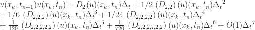
When solved using the Lax-Wendroff scheme, it is expressed as

$u(x_{{k}},t_{{n+1}})=u(x_{{k}},t_{{n}})-1/2\, R\left(u(x_{{k+1}},t_{{n}})-u(x_{{k-1}},t_{{n}})\right)\\+1/2\,{R}^{2}\left(u(x_{{k+1}},t_{{n}})-2\, u(x_{{k}},t_{{n}})+u(x_{{k-1}},t_{{n}})\right)$

where

$R=a\frac{\Delta_{t}}{\Delta_{x}}$

The solution for this problem is given in Numerical Methods for Engineers and Scientists, Second Edition.

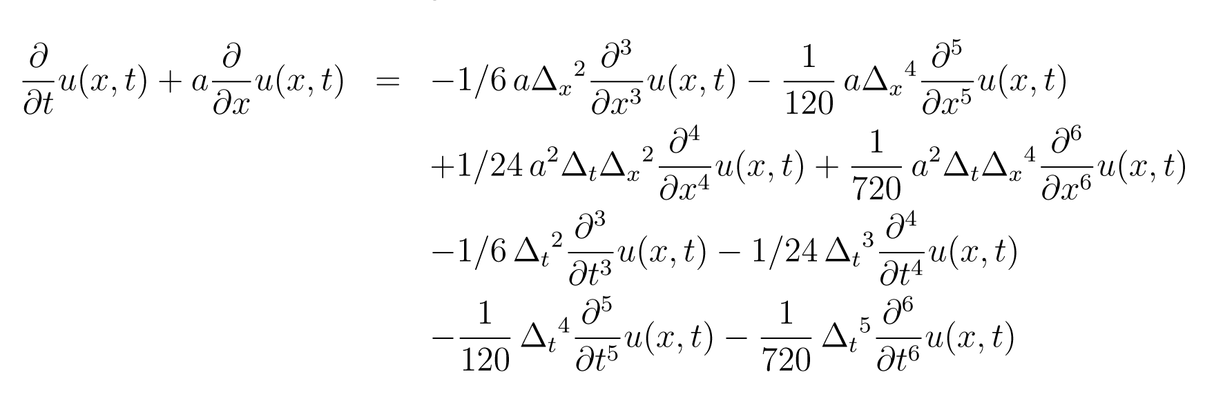
Application of Taylor Series Expansions for Consistency

If we apply the results of the Taylor series expansions to the Lax-Wendroff scheme and perform a good deal of algebra (including substituting for $R$ ,) the result is

$u(x_{{k}},t_{{n}})+D_{{2}}(u)(x_{{k}},t_{{n}})\Delta_{{t}}+1/2\,\left(D_{{2,2}}\right)(u)(x_{{k}},t_{{n}}){\Delta_{{t}}}^{2}+1/6\,\left(D_{{2,2,2}}\right)(u)(x_{{k}},t_{{n}}){\Delta_{{t}}}^{3}\\+1/24\,\left(D_{{2,2,2,2}}\right)(u)(x_{{k}},t_{{n}}){\Delta_{{t}}}^{4}+{\frac{1}{120}}\,\left(D_{{2,2,2,2,2}}\right)(u)(x_{{k}},t_{{n}}){\Delta_{{t}}}^{5}+{\frac{1}{720}}\,\left(D_{{2,2,2,2,2,2}}\right)(u)(x_{{k}},t_{{n}}){\Delta_{{t}}}^{6}+O(1){\Delta_{{t}}}^{7}\\=\\u(x_{{k}},t_{{n}})+r\left(D_{{1,1}}\right)(u)(x_{{k}},t_{{n}}){\Delta_{{x}}}^{2}-1/12\, r\left(D_{{1,1,1,1}}\right)(u)(x_{{k}},t_{{n}}){\Delta_{{x}}}^{4}-1/40\, r\left(D_{{1,1,1,1,1,1}}\right)(u)(x_{{k}},t_{{n}}){\Delta_{{x}}}^{6}$

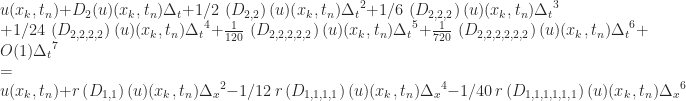
Rearranging, making a change in notation and dropping the $\mathcal{O}$ terms as well,

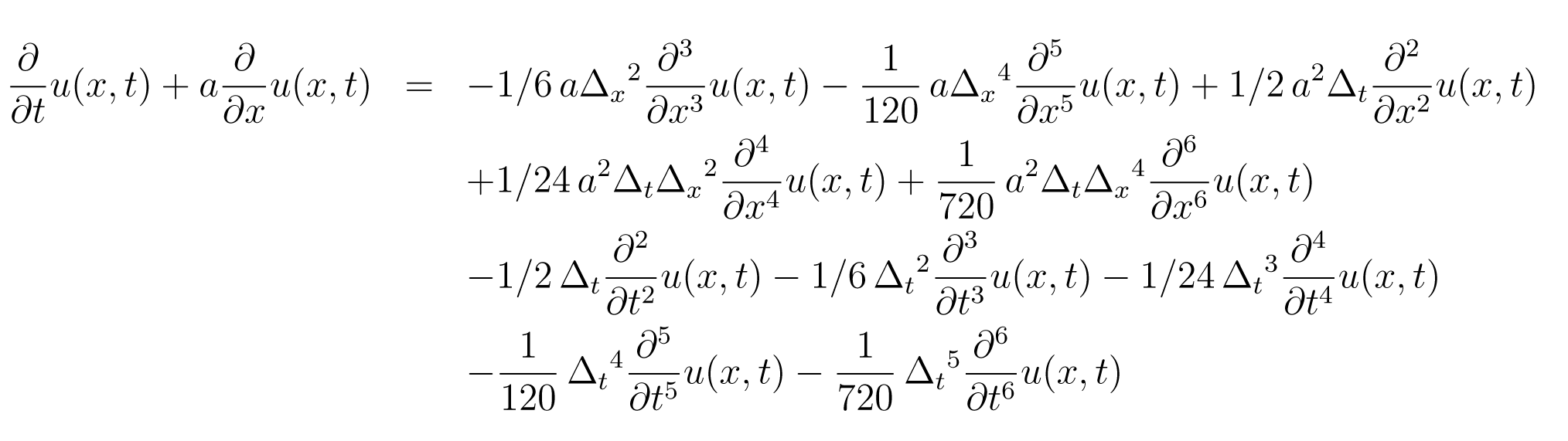
On the left hand side is the exact equation, which is strictly speaking equal to zero. On the right hand side is the residual for consistency of the finite difference scheme. If the scheme is consistent with the original equation, it too should approach zero as $\Delta_{x},\,\Delta_{t}\rightarrow0$ . Based on this we note the following:

All of the right hand side terms contain $\Delta_{x},\,\Delta_{t}$ or both. Thus, as these approach zero, the entire right hand side will approach zero. Thus the scheme is consistent with the original differential equation.
The lowest order terms for the time and spatial steps on the right hand side are $\Delta_{t}$ and $\Delta_{x}^{2}$ respectively. Thus we can conclude that the truncation error is $\mathcal{O}\left(t\right)+\mathcal{O}\left(x^{2}\right)$ .

Or is it? Let us assume that the solution is twice differentiable. By this we mean that the function has second derivatives in both space and time. (Another way of interpreting this is to say that “twice differentiable” means that the solution has no derivatives beyond the second, in which case many of the terms in the Taylor Series expansion would go to zero.) Then we differentiate the original equation once temporally, thus

${\frac{\partial^{2}}{\partial{t}^{2}}}v(x,t)+a{\frac{\partial^{2}}{\partial t\partial x}}v(x,t)=0$

Now let us do the same thing but spatially, and (with a little additional algebra) we obtain

$-a{\frac{\partial^{2}}{\partial t\partial x}}v(x,t)-{a}^{2}{\frac{\partial^{2}}{\partial{x}^{2}}}v(x,t)=0$

Adding these two, we have

${\frac{\partial^{2}}{\partial{t}^{2}}}v(x,t)-{a}^{2}{\frac{\partial^{2}}{\partial{x}^{2}}}v(x,t)=0$

which is, mirabile visu, the wave equation. Applying this solution for the original equation to the finite difference residual results in

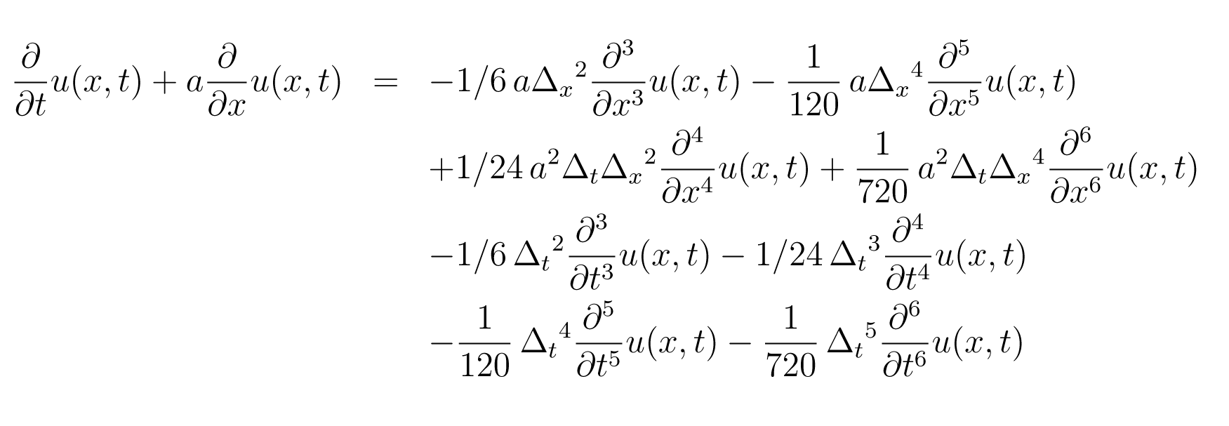
Now we see that the lowest order terms are $\Delta_{t}^{2}$ and $\Delta_{x}^{2}$ , which means that the truncation error is $\mathcal{O}\left(t^{2}\right)+\mathcal{O}\left(x^{2}\right)$ . We duly note that the fourth order spatial derivative is multiplied by $\Delta_{{t}}{\Delta_{{x}}}^{2}$ . However, the squared term will be the predominant one as $\Delta_{x},\,\Delta_{t}\rightarrow0$ , so this does not change our conclusion. Also, if “twice differentiable” means that the function has no further derivatives beyond the second, then all of the terms go to zero, and the numerical solution, within machine accuracy, is exact. This also applies to the next section as well; the vector described there would be the zero vector under these conditions.

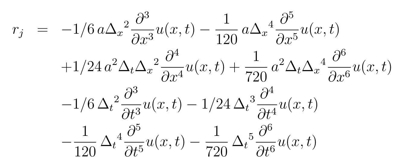
Consistency in a Norm

The Taylor Series expansion is only valid at the point at which it is taken. For most differential equations, we are interested in solutions along a broader region. This is in part the purpose for considering consistency in a norm.

Let us consider the result we just obtained, thus

The right hand side represents the residual for consistency of the finite difference scheme. If we were to consider a Taylor Series expansion for all of the points in space and time under consideration, what we would end up with is an infinite set of residuals, i.e., the right hand side of the above equation, which could then be arranged in a vector. If we designate this vector as $R$ , then each entry can be designated as follows:

Now let us consider the nature of the differential equation. The following is adapted from Numerical Solution of Differential Equations: Finite Difference and Finite Element Solution of the Initial, Boundary and Eigenvalue Problem in the… (Computer Science and Applied Mathematics).

We can consider the differential equation as a linear transformation. Since we have defined the results as an vector, we can express this as follows for the exact solution:

$Av\left(x,t\right)=F$

and for the finite difference solution

$Au\left(x,t\right)=F+R$

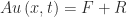
The result difference between the two is the residual we defined earlier. The finite difference representation is the same as the original if and only if $A$ is the same in both cases. Combining both equations,

$A\left(v\left(x,t\right)-u\left(x,t\right)\right)=R$

and rearranging

$v\left(x,t\right)-u\left(x,t\right)=A^{-1}R$

Now let us consider the norm. Given the infinite number of entries in this vector, the most convenient norm to take would be the infinity norm, where the norm would be the largest absolute value in the set. For an inner product space,

$||v\left(x,t\right)-u\left(x,t\right)||_{\infty}=||A^{-1}||_{\infty}\,||R||_{\infty}$

We have shown that each and every $r_{n}\rightarrow0$ as $\Delta_{x},\,\Delta_{t}\rightarrow0$ . (Additionally the function would have to be bounded, continuous and at least twice differentiable at all points.) From this, $R\rightarrow0$ and $||R||_{\infty}\rightarrow0$ . If $A$ and $A^{-1}$ are bounded (as they are in a linear transformation,) then $||v\left(x,t\right)-u\left(x,t\right)||_{\infty}\rightarrow0$ and thus the exact solution and its finite difference counterpart become the same. This is consistency by definition. (The most serious obstacle to actually constructing such a vector–a necessary prerequisite to a norm–is evaluating the derivatives. One “solution” would be to used the exact solution of the original differential equation, but that assumes we can arrive at an exact solution. In many cases, the whole point of a numerical solution is because the exact, “closed form” solution is unavailable. Thus we would end up with numerical evaluations for the derivatives.)

As for other norms such as the Euclidean norm, if the entries in the vector approach zero as $\Delta_{x},\,\Delta_{t}\rightarrow0$ , we would expect the norm to do so as well, as discussed above. It should be noted that the infinity norm would be best to pick up a point slowly converging on zero than a Euclidean norm.

von Neumann Stability Analysis

Turning to the issue of stability, we will perform a von Neumann analysis. In this type of analysis we will analyze a stability factor $|G|$ defined as follows:

$1\geq|G|=\frac{u(x_{{k}},t_{{n+1}})}{u(x_{{k}},t_{{n}})}$

The idea behind this is to determine “whether or not the calculation can be rendered useless by unfavourable error propagation” (from The Numerical Treatment of Differential Equations.) In other methods, such as perturbation methods, an error is introduced into the scheme and its propagation is explicitly analysed. The von Neumann analysis does the same thing but in a more compact form.

The heart of the von Neumann method is to substitute a Fourier series expression into the difference scheme. Thus, for our difference scheme

$u(x_{{k}},t_{{n+1}})=u(x_{{k}},t_{{n}})-1/2\, R\left(u(x_{{k+1}},t_{{n}})-u(x_{{k-1}},t_{{n}})\right)+1/2\,{R}^{2}\left(u(x_{{k+1}},t_{{n}})-2\, u(x_{{k}},t_{{n}})+u(x_{{k-1}},t_{{n}})\right)$

we substitute
$u(x_{{k}},t_{{n+1}})={e^{p_{{m}}\left(t+\Delta_{{t}}\right)+\sqrt{-1}k_{{m}}x}}\\u(x_{{k}},t_{{n}})={e^{p_{{m}}t+\sqrt{-1}k_{{m}}x}}\\u(x_{{k+1}},t_{{n}})={e^{p_{{m}}t+\sqrt{-1}k_{{m}}\left(x+\Delta_{{x}}\right)}}\\u(x_{{k-1}},t_{{n}})= {e^{p_{{m}}t+\sqrt{-1}k_{{m}}\left(x-\Delta_{{x}}\right)}}$

to yield

${e^{p_{{m}}\left(t+\Delta_{{t}}\right)+\sqrt{-1}k_{{m}}x}}={e^{p_{{m}}t+\sqrt{-1}k_{{m}}x}}\\-1/2\, R\left({e^{p_{{m}}t+\sqrt{-1}k_{{m}}\left(x+\Delta_{{x}}\right)}}-{e^{p_{{m}}t+\sqrt{-1}k_{{m}}\left(x-\Delta_{{x}}\right)}}\right)\\+1/2\,{R}^{2}\left({e^{p_{{m}}t+\sqrt{-1}k_{{m}}\left(x+\Delta_{{x}}\right)}}-2\,{e^{p_{{m}}t+\sqrt{-1}k_{{m}}x}}+{e^{p_{{m}}t+\sqrt{-1}k_{{m}}\left(x-\Delta_{{x}}\right)}}\right)$

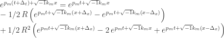
As an aside, When most people think of “Fourier series” they think of a real series of sines, cosines and coefficients. This was certainly in evidence in the presentation of the method in The Numerical Treatment of Differential Equations. However, it has been the author’s experience that the best way to treat these is to do so in a “real-complex continuum,” i.e., to express these exponentially and to convert them to circular (or in some cases hyperbolic) functions as the complex analysis would admit. An example of that is here.

Solving for the amplification factor defined above,

$|G|={\frac{{e^{p_{{m}}t+\sqrt{-1}k_{{m}}x}}-1/2\, R\left({e^{p_{{m}}t+\sqrt{-1}k_{{m}}\left(x+\Delta_{{x}}\right)}}-{e^{p_{{m}}t+\sqrt{-1}k_{{m}}\left(x-\Delta_{{x}}\right)}}\right)}{{e^{p_{{m}}t+\sqrt{-1}k_{{m}}x}}}}\\+{\frac{1/2\,{R}^{2}\left({e^{p_{{m}}t+\sqrt{-1}k_{{m}}\left(x+\Delta_{{x}}\right)}}-2\,{e^{p_{{m}}t+\sqrt{-1}k_{{m}}x}}+{e^{p_{{m}}t+\sqrt{-1}k_{{m}}\left(x-\Delta_{{x}}\right)}}\right)}{{e^{p_{{m}}t+\sqrt{-1}k_{{m}}x}}}}$

Simplifying,
$|G|=1-1/2\, R{e^{\sqrt{-1}k_{{m}}\Delta_{{x}}}}+1/2\, R{e^{-\sqrt{-1}k_{{m}}\Delta_{{x}}}}+1/2\,{R}^{2}{e^{\sqrt{-1}k_{{m}}\Delta_{{x}}}}-{R}^{2}+1/2\,{R}^{2}{e^{-\sqrt{-1}k_{{m}}\Delta_{{x}}}}$

or
$|G|=1+{R}^{2}\cos(k_{{m}}\Delta_{{x}})-{R}^{2}-\sqrt{-1}R\sin(k_{{m}}\Delta_{{x}})$

and then

$1\geq G=\sqrt{\left(1+{R}^{2}\cos(k_{{m}}\Delta_{{x}})-{R}^{2}\right)^{2}+{R}^{2}\left(\sin(k_{{m}}\Delta_{{x}})\right)^{2}}$

Solving for $R$ at the points of equality yields three results: $R=-1,0,1$ . Since negative values for $R$ have no physical meaning, we conclude that

$0\leq R\leq1$

for this method to be stable. Thus we can say that the method is conditionally unstable.

Convergence

The Lax Equivalence Theorem posits that, if the problem is properly posed and the finite difference scheme used is consistent and stable, the necessary and consistent conditions for convergence have been met (see Numerical Methods for Engineers and Scientists, Second Edition.) We have shown that, with the assumptions stated above, the scheme is consistent with the original differential equation, with or without the provision of twice differentiability. The method is thus convergent within the conditions stated above for stability; outside of those conditions the method is neither stable nor convergent.

Overview of Taylor Series Expansions

Convection Equation

Application of Taylor Series Expansions for Consistency

Consistency in a Norm

von Neumann Stability Analysis

Convergence

Share this:

Like this:

Related

Leave a Reply Cancel reply