Local Stiffness Matrix for Combined Beam and Spar Element With Axial and Lateral Linear Resistance

Our objective is to develop an element with the following characteristics:

Two-dimensional, two node element
Euler-Bernoulli beam theory
Axial stiffness (“spar” type element)
“Beam on elastic foundation” characteristic
Axial elastic resistance

Although it is doubtless possible to start with a single weak-form equation and develop the stiffness matrix, it is more convenient to develop the axial and bending local stiffness matrices separately and then to put them together with superposition.

Both spar and beam elements generally use two nodes, one at each end. For this derivation all of the constants (beam elastic modulus, moment of inertia, cross-sectional area and spring constants) will be assumed to be uniform the full length of the element. If one desires to model non-uniform beams, one can either develop an element with the desired non-uniformity or use more elements, and we see both in finite element analysis.

Let us start with the bending portion. The weak form of the equation for the fourth-order Euler-Bernoulli beam element is
$\int_{x_{{1}}}^{x_{{2}}}\!{\it E1}\,{\it XI1}\,\left({\frac{d^{2}}{d{x}^{2}}}v(x)\right){\frac{d^{2}}{d{x}^{2}}}w(x)+gv(x)w(x)-v(x)t{dx}=0$

where $E1$ is the Young’s modulus of the material and $XI1$ is the moment of inertia of the beam. The variable $g$ represents the continuous spring constant along the length of the beam relative to the displacement of that beam, the “beam on elastic foundation.” The variable $t$ is a uniform load along the beam. The equations were derived using Maple with the idea of the results used on FORTRAN 77, thus the naming convention of some of the variables. An explanation of the weak form, its derivation and the significance of $w\left(x\right)$ and $v\left(x\right)$ can be found in a finite element text such as this.

At this point we need to select appropriate weighting functions for the equation. For beam elements we choose weighting functions to satisfy the Hermite interplation of the two primary variables at local nodes 1 and 2, to wit

$\Delta_{{1}}=C_{{1}}+C_{{2}}x_{{1}}+C_{{3}}{x_{{1}}}^{2}+C_{{4}}{x_{{1}}}^{3}$
$\Delta_{{2}}=-C_{{2}}-2\, C_{{3}}x_{{1}}-3\, C_{{4}}{x_{{1}}}^{2}$
$\Delta_{{3}}=C_{{1}}+C_{{2}}x_{{2}}+C_{{3}}{x_{{2}}}^{2}+C_{{4}}{x_{{2}}}^{3}$
$\Delta_{{4}}=-C_{{2}}-2\, C_{{3}}x_{{2}}-3\, C_{{4}}{x_{{2}}}^{2}$

where $\Delta_{1},\,\Delta_{3}$ are the “displacements” for nodes
1 and 2 and $\Delta_{2},\,\Delta_{4}$ are the first derivative slopes
at these nodes.

This can be expressed in matrix form as follows:

$\left[\begin{array}{cccc} 1 & x_{{1}} & {x_{{1}}}^{2} & {x_{{1}}}^{3}\\ \noalign{\medskip}0 & -1 & -2\, x_{{1}} & -3\,{x_{{1}}}^{2}\\ \noalign{\medskip}1 & x_{{2}} & {x_{{2}}}^{2} & {x_{{2}}}^{3}\\ \noalign{\medskip}0 & -1 & -2\, x_{{2}} & -3\,{x_{{2}}}^{2} \end{array}\right]\left[\begin{array}{c} C_{{1}}\\ \noalign{\medskip}C_{{2}}\\ \noalign{\medskip}C_{{3}}\\ \noalign{\medskip}C_{{4}} \end{array}\right]=\left[\begin{array}{c} \Delta_{{1}}\\ \noalign{\medskip}\Delta_{{2}}\\ \noalign{\medskip}\Delta_{{3}}\\ \noalign{\medskip}\Delta_{{4}} \end{array}\right]$

Inverting the matrix, we have

$\left[\begin{array}{c} C_{{1}}\\ \noalign{\medskip}C_{{2}}\\ \noalign{\medskip}C_{{3}}\\ \noalign{\medskip}C_{{4}} \end{array}\right]=\left[\begin{array}{cccc} {\frac{\left(3\, x_{{1}}-x_{{2}}\right){x_{{2}}}^{2}}{{x_{{1}}}^{3}-3\,{x_{{1}}}^{2}x_{{2}}+3\, x_{{1}}{x_{{2}}}^{2}-{x_{{2}}}^{3}}} & {\frac{x_{{1}}{x_{{2}}}^{2}}{{x_{{2}}}^{2}-2\, x_{{1}}x_{{2}}+{x_{{1}}}^{2}}} & {\frac{\left(x_{{1}}-3\, x_{{2}}\right){x_{{1}}}^{2}}{{x_{{1}}}^{3}-3\,{x_{{1}}}^{2}x_{{2}}+3\, x_{{1}}{x_{{2}}}^{2}-{x_{{2}}}^{3}}} & {\frac{{x_{{1}}}^{2}x_{{2}}}{{x_{{2}}}^{2}-2\, x_{{1}}x_{{2}}+{x_{{1}}}^{2}}}\\ \noalign{\medskip}-6\,{\frac{x_{{1}}x_{{2}}}{{x_{{1}}}^{3}-3\,{x_{{1}}}^{2}x_{{2}}+3\, x_{{1}}{x_{{2}}}^{2}-{x_{{2}}}^{3}}} & -{\frac{\left(2\, x_{{1}}+x_{{2}}\right)x_{{2}}}{{x_{{2}}}^{2}-2\, x_{{1}}x_{{2}}+{x_{{1}}}^{2}}} & 6\,{\frac{x_{{1}}x_{{2}}}{{x_{{1}}}^{3}-3\,{x_{{1}}}^{2}x_{{2}}+3\, x_{{1}}{x_{{2}}}^{2}-{x_{{2}}}^{3}}} & -{\frac{\left(x_{{1}}+2\, x_{{2}}\right)x_{{1}}}{{x_{{2}}}^{2}-2\, x_{{1}}x_{{2}}+{x_{{1}}}^{2}}}\\ \noalign{\medskip}3\,{\frac{x_{{1}}+x_{{2}}}{{x_{{1}}}^{3}-3\,{x_{{1}}}^{2}x_{{2}}+3\, x_{{1}}{x_{{2}}}^{2}-{x_{{2}}}^{3}}} & {\frac{x_{{1}}+2\, x_{{2}}}{{x_{{2}}}^{2}-2\, x_{{1}}x_{{2}}+{x_{{1}}}^{2}}} & -3\,{\frac{x_{{1}}+x_{{2}}}{{x_{{1}}}^{3}-3\,{x_{{1}}}^{2}x_{{2}}+3\, x_{{1}}{x_{{2}}}^{2}-{x_{{2}}}^{3}}} & {\frac{2\, x_{{1}}+x_{{2}}}{{x_{{2}}}^{2}-2\, x_{{1}}x_{{2}}+{x_{{1}}}^{2}}}\\ \noalign{\medskip}-2\,\left({x_{{1}}}^{3}-3\,{x_{{1}}}^{2}x_{{2}}+3\, x_{{1}}{x_{{2}}}^{2}-{x_{{2}}}^{3}\right)^{-1} & -\left({x_{{2}}}^{2}-2\, x_{{1}}x_{{2}}+{x_{{1}}}^{2}\right)^{-1} & 2\,\left({x_{{1}}}^{3}-3\,{x_{{1}}}^{2}x_{{2}}+3\, x_{{1}}{x_{{2}}}^{2}-{x_{{2}}}^{3}\right)^{-1} & -\left({x_{{2}}}^{2}-2\, x_{{1}}x_{{2}}+{x_{{1}}}^{2}\right)^{-1} \end{array}\right]\left[\begin{array}{c} \Delta_{{1}}\\ \noalign{\medskip}\Delta_{{2}}\\ \noalign{\medskip}\Delta_{{3}}\\ \noalign{\medskip}\Delta_{{4}} \end{array}\right]$
Multiplying the result, we have for the coefficients
$\left[\begin{array}{c} C_{{1}}\\ \noalign{\medskip}C_{{2}}\\ \noalign{\medskip}C_{{3}}\\ \noalign{\medskip}C_{{4}} \end{array}\right]=\left[\begin{array}{c} {\frac{\left(3\, x_{{1}}-x_{{2}}\right){x_{{2}}}^{2}\Delta_{{1}}}{{x_{{1}}}^{3}-3\,{x_{{1}}}^{2}x_{{2}}+3\, x_{{1}}{x_{{2}}}^{2}-{x_{{2}}}^{3}}}+{\frac{x_{{1}}{x_{{2}}}^{2}\Delta_{{2}}}{{x_{{2}}}^{2}-2\, x_{{1}}x_{{2}}+{x_{{1}}}^{2}}}+{\frac{\left(x_{{1}}-3\, x_{{2}}\right){x_{{1}}}^{2}\Delta_{{3}}}{{x_{{1}}}^{3}-3\,{x_{{1}}}^{2}x_{{2}}+3\, x_{{1}}{x_{{2}}}^{2}-{x_{{2}}}^{3}}}+{\frac{{x_{{1}}}^{2}x_{{2}}\Delta_{{4}}}{{x_{{2}}}^{2}-2\, x_{{1}}x_{{2}}+{x_{{1}}}^{2}}}\\ \noalign{\medskip}-6\,{\frac{x_{{1}}x_{{2}}\Delta_{{1}}}{{x_{{1}}}^{3}-3\,{x_{{1}}}^{2}x_{{2}}+3\, x_{{1}}{x_{{2}}}^{2}-{x_{{2}}}^{3}}}-{\frac{\left(2\, x_{{1}}+x_{{2}}\right)x_{{2}}\Delta_{{2}}}{{x_{{2}}}^{2}-2\, x_{{1}}x_{{2}}+{x_{{1}}}^{2}}}+6\,{\frac{x_{{1}}x_{{2}}\Delta_{{3}}}{{x_{{1}}}^{3}-3\,{x_{{1}}}^{2}x_{{2}}+3\, x_{{1}}{x_{{2}}}^{2}-{x_{{2}}}^{3}}}-{\frac{\left(x_{{1}}+2\, x_{{2}}\right)x_{{1}}\Delta_{{4}}}{{x_{{2}}}^{2}-2\, x_{{1}}x_{{2}}+{x_{{1}}}^{2}}}\\ \noalign{\medskip}3\,{\frac{\left(x_{{1}}+x_{{2}}\right)\Delta_{{1}}}{{x_{{1}}}^{3}-3\,{x_{{1}}}^{2}x_{{2}}+3\, x_{{1}}{x_{{2}}}^{2}-{x_{{2}}}^{3}}}+{\frac{\left(x_{{1}}+2\, x_{{2}}\right)\Delta_{{2}}}{{x_{{2}}}^{2}-2\, x_{{1}}x_{{2}}+{x_{{1}}}^{2}}}-3\,{\frac{\left(x_{{1}}+x_{{2}}\right)\Delta_{{3}}}{{x_{{1}}}^{3}-3\,{x_{{1}}}^{2}x_{{2}}+3\, x_{{1}}{x_{{2}}}^{2}-{x_{{2}}}^{3}}}+{\frac{\left(2\, x_{{1}}+x_{{2}}\right)\Delta_{{4}}}{{x_{{2}}}^{2}-2\, x_{{1}}x_{{2}}+{x_{{1}}}^{2}}}\\ \noalign{\medskip}-2\,{\frac{\Delta_{{1}}}{{x_{{1}}}^{3}-3\,{x_{{1}}}^{2}x_{{2}}+3\, x_{{1}}{x_{{2}}}^{2}-{x_{{2}}}^{3}}}-{\frac{\Delta_{{2}}}{{x_{{2}}}^{2}-2\, x_{{1}}x_{{2}}+{x_{{1}}}^{2}}}+2\,{\frac{\Delta_{{3}}}{{x_{{1}}}^{3}-3\,{x_{{1}}}^{2}x_{{2}}+3\, x_{{1}}{x_{{2}}}^{2}-{x_{{2}}}^{3}}}-{\frac{\Delta_{{4}}}{{x_{{2}}}^{2}-2\, x_{{1}}x_{{2}}+{x_{{1}}}^{2}}} \end{array}\right]$

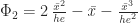
The weighting function in its complete form is thus

$w={\frac{\left(3\, x_{{1}}-x_{{2}}\right){x_{{2}}}^{2}\Delta_{{1}}}{{x_{{1}}}^{3}-3\,{x_{{1}}}^{2}x_{{2}}+3\, x_{{1}}{x_{{2}}}^{2}-{x_{{2}}}^{3}}}+{\frac{x_{{1}}{x_{{2}}}^{2}\Delta_{{2}}}{{x_{{2}}}^{2}-2\, x_{{1}}x_{{2}}+{x_{{1}}}^{2}}}+{\frac{\left(x_{{1}}-3\, x_{{2}}\right){x_{{1}}}^{2}\Delta_{{3}}}{{x_{{1}}}^{3}-3\,{x_{{1}}}^{2}x_{{2}}+3\, x_{{1}}{x_{{2}}}^{2}-{x_{{2}}}^{3}}}+{\frac{{x_{{1}}}^{2}x_{{2}}\Delta_{{4}}}{{x_{{2}}}^{2}-2\, x_{{1}}x_{{2}}+{x_{{1}}}^{2}}}+$

$-6\,{\frac{x_{{1}}x_{{2}}\Delta_{{1}}}{{x_{{1}}}^{3}-3\,{x_{{1}}}^{2}x_{{2}}+3\, x_{{1}}{x_{{2}}}^{2}-{x_{{2}}}^{3}}}x-{\frac{\left(2\, x_{{1}}+x_{{2}}\right)x_{{2}}\Delta_{{2}}}{{x_{{2}}}^{2}-2\, x_{{1}}x_{{2}}+{x_{{1}}}^{2}}}x+6\,{\frac{x_{{1}}x_{{2}}\Delta_{{3}}}{{x_{{1}}}^{3}-3\,{x_{{1}}}^{2}x_{{2}}+3\, x_{{1}}{x_{{2}}}^{2}-{x_{{2}}}^{3}}}x-{\frac{\left(x_{{1}}+2\, x_{{2}}\right)x_{{1}}\Delta_{{4}}}{{x_{{2}}}^{2}-2\, x_{{1}}x_{{2}}+{x_{{1}}}^{2}}}x$

$3\,{\frac{\left(x_{{1}}+x_{{2}}\right)\Delta_{{1}}}{{x_{{1}}}^{3}-3\,{x_{{1}}}^{2}x_{{2}}+3\, x_{{1}}{x_{{2}}}^{2}-{x_{{2}}}^{3}}}{x}^{2}+{\frac{\left(x_{{1}}+2\, x_{{2}}\right)\Delta_{{2}}}{{x_{{2}}}^{2}-2\, x_{{1}}x_{{2}}+{x_{{1}}}^{2}}}{x}^{2}-3\,{\frac{\left(x_{{1}}+x_{{2}}\right)\Delta_{{3}}}{{x_{{1}}}^{3}-3\,{x_{{1}}}^{2}x_{{2}}+3\, x_{{1}}{x_{{2}}}^{2}-{x_{{2}}}^{3}}}{x}^{2}+{\frac{\left(2\, x_{{1}}+x_{{2}}\right)\Delta_{{4}}}{{x_{{2}}}^{2}-2\, x_{{1}}x_{{2}}+{x_{{1}}}^{2}}}{x}^{2}$

$-2\,{\frac{\Delta_{{1}}}{{x_{{1}}}^{3}-3\,{x_{{1}}}^{2}x_{{2}}+3\, x_{{1}}{x_{{2}}}^{2}-{x_{{2}}}^{3}}}{x}^{3}-{\frac{\Delta_{{2}}}{{x_{{2}}}^{2}-2\, x_{{1}}x_{{2}}+{x_{{1}}}^{2}}}{x}^{3}+2\,{\frac{\Delta_{{3}}}{{x_{{1}}}^{3}-3\,{x_{{1}}}^{2}x_{{2}}+3\, x_{{1}}{x_{{2}}}^{2}-{x_{{2}}}^{3}}}{x}^{3}-{\frac{\Delta_{{4}}}{{x_{{2}}}^{2}-2\, x_{{1}}x_{{2}}+{x_{{1}}}^{2}}}{x}^{3}$

This breaks down in to weighting functions for each independent variable as follows:
$\Phi_{1}=1-3\,{\frac{{\it \bar{x}}^{2}}{{\it he}^{2}}}+2\,{\frac{{\it \bar{x}}^{3}}{{\it he}^{3}}}$

$\Phi_{2}=2\,{\frac{{\it \bar{x}}^{2}}{{\it he}}}-{\it \bar{x}}-{\frac{{\it \bar{x}}^{3}}{{\it he}^{2}}}$

$\Phi_{3}=3\,{\frac{{\it \bar{x}}^{2}}{{\it he}^{2}}}-2\,{\frac{{\it \bar{x}}^{3}}{{\it he}^{3}}}$

$\Phi_{4}=-{\frac{{\it \bar{x}}^{3}}{{\it he}^{2}}}+{\frac{{\it \bar{x}}^{2}}{{\it he}}}$

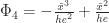
additionally assuming that

$\bar{x}=x-x_{1}$
$he=x_{2}-x_{1}$

If we substitute these weighting functions into the weak form of the governing equations, perform the appropriate substitution, differentiation, integration and algebra, the first term results in the following stiffness matrix:

$M=\left[\begin{array}{cccc} 12\,{\frac{{\it E1}\,{\it XI1}}{{\it he}^{3}}} & -6\,{\frac{{\it E1}\,{\it XI1}}{{\it he}^{2}}} & -12\,{\frac{{\it E1}\,{\it XI1}}{{\it he}^{3}}} & -6\,{\frac{{\it E1}\,{\it XI1}}{{\it he}^{2}}}\\ \noalign{\medskip}-6\,{\frac{{\it E1}\,{\it XI1}}{{\it he}^{2}}} & 4\,{\frac{{\it E1}\,{\it XI1}}{{\it he}}} & 6\,{\frac{{\it E1}\,{\it XI1}}{{\it he}^{2}}} & 2\,{\frac{{\it E1}\,{\it XI1}}{{\it he}}}\\ \noalign{\medskip}-12\,{\frac{{\it E1}\,{\it XI1}}{{\it he}^{3}}} & 6\,{\frac{{\it E1}\,{\it XI1}}{{\it he}^{2}}} & 12\,{\frac{{\it E1}\,{\it XI1}}{{\it he}^{3}}} & 6\,{\frac{{\it E1}\,{\it XI1}}{{\it he}^{2}}}\\ \noalign{\medskip}-6\,{\frac{{\it E1}\,{\it XI1}}{{\it he}^{2}}} & 2\,{\frac{{\it E1}\,{\it XI1}}{{\it he}}} & 6\,{\frac{{\it E1}\,{\it XI1}}{{\it he}^{2}}} & 4\,{\frac{{\it E1}\,{\it XI1}}{{\it he}}} \end{array}\right]$

The second term (for the “elastic foundation”) yields the following stiffness matrix:
$N=\left[\begin{array}{cccc} {\frac{13}{35}}\,{\it he}\, g & -{\frac{11}{210}}\,{\it he}^{2}g & {\frac{9}{70}}\,{\it he}\, g & {\frac{13}{420}}\,{\it he}^{2}g\\ \noalign{\medskip}-{\frac{11}{210}}\,{\it he}^{2}g & {\frac{1}{105}}\,{\it he}^{3}g & -{\frac{13}{420}}\,{\it he}^{2}g & -{\frac{1}{140}}\,{\it he}^{3}g\\ \noalign{\medskip}{\frac{9}{70}}\,{\it he}\, g & -{\frac{13}{420}}\,{\it he}^{2}g & {\frac{13}{35}}\,{\it he}\, g & {\frac{11}{210}}\,{\it he}^{2}g\\ \noalign{\medskip}{\frac{13}{420}}\,{\it he}^{2}g & -{\frac{1}{140}}\,{\it he}^{3}g & {\frac{11}{210}}\,{\it he}^{2}g & {\frac{1}{105}}\,{\it he}^{3}g \end{array}\right]$

The combined local stiffness matrix for bending only is

$K_{b}=\left[\begin{array}{cccc} 12\,{\frac{{\it E1}\,{\it XI1}}{{\it he}^{3}}}+{\frac{13}{35}}\,{\it he}\, g & -6\,{\frac{{\it E1}\,{\it XI1}}{{\it he}^{2}}}-{\frac{11}{210}}\,{\it he}^{2}g & -12\,{\frac{{\it E1}\,{\it XI1}}{{\it he}^{3}}}+{\frac{9}{70}}\,{\it he}\, g & -6\,{\frac{{\it E1}\,{\it XI1}}{{\it he}^{2}}}+{\frac{13}{420}}\,{\it he}^{2}g\\ \noalign{\medskip}-6\,{\frac{{\it E1}\,{\it XI1}}{{\it he}^{2}}}-{\frac{11}{210}}\,{\it he}^{2}g & 4\,{\frac{{\it E1}\,{\it XI1}}{{\it he}}}+{\frac{1}{105}}\,{\it he}^{3}g & 6\,{\frac{{\it E1}\,{\it XI1}}{{\it he}^{2}}}-{\frac{13}{420}}\,{\it he}^{2}g & 2\,{\frac{{\it E1}\,{\it XI1}}{{\it he}}}-{\frac{1}{140}}\,{\it he}^{3}g\\ \noalign{\medskip}-12\,{\frac{{\it E1}\,{\it XI1}}{{\it he}^{3}}}+{\frac{9}{70}}\,{\it he}\, g & 6\,{\frac{{\it E1}\,{\it XI1}}{{\it he}^{2}}}-{\frac{13}{420}}\,{\it he}^{2}g & 12\,{\frac{{\it E1}\,{\it XI1}}{{\it he}^{3}}}+{\frac{13}{35}}\,{\it he}\, g & 6\,{\frac{{\it E1}\,{\it XI1}}{{\it he}^{2}}}+{\frac{11}{210}}\,{\it he}^{2}g\\ \noalign{\medskip}-6\,{\frac{{\it E1}\,{\it XI1}}{{\it he}^{2}}}+{\frac{13}{420}}\,{\it he}^{2}g & 2\,{\frac{{\it E1}\,{\it XI1}}{{\it he}}}-{\frac{1}{140}}\,{\it he}^{3}g & 6\,{\frac{{\it E1}\,{\it XI1}}{{\it he}^{2}}}+{\frac{11}{210}}\,{\it he}^{2}g & 4\,{\frac{{\it E1}\,{\it XI1}}{{\it he}}}+{\frac{1}{105}}\,{\it he}^{3}g \end{array}\right]$

The FORTRAN 77 code for this is as follows:

K(1,1) = 12/he**3*E1*XI1+13.E0/35.E0*he*g
K(1,2) = -6/he**2*E1*XI1-11.E0/210.E0*he**2*g
K(1,3) = -12/he**3*E1*XI1+9.E0/70.E0*he*g
K(1,4) = -6/he**2*E1*XI1+13.E0/420.E0*he**2*g
K(2,1) = -6/he**2*E1*XI1-11.E0/210.E0*he**2*g
K(2,2) = 4/he*E1*XI1+he**3*g/105
K(2,3) = 6/he**2*E1*XI1-13.E0/420.E0*he**2*g
K(2,4) = 2/he*E1*XI1-he**3*g/140
K(3,1) = -12/he**3*E1*XI1+9.E0/70.E0*he*g
K(3,2) = 6/he**2*E1*XI1-13.E0/420.E0*he**2*g
K(3,3) = 12/he**3*E1*XI1+13.E0/35.E0*he*g
K(3,4) = 6/he**2*E1*XI1+11.E0/210.E0*he**2*g
K(4,1) = -6/he**2*E1*XI1+13.E0/420.E0*he**2*g
K(4,2) = 2/he*E1*XI1-he**3*g/140
K(4,3) = 6/he**2*E1*XI1+11.E0/210.E0*he**2*g
K(4,4) = 4/he*E1*XI1+he**3*g/105

The vector for the last term is

$T=\left[\begin{array}{c} 1/2\,{\it he}\, t\\ \noalign{\medskip}-1/12\,{\it he}^{2}t\\ \noalign{\medskip}1/2\,{\it he}\, t\\ \noalign{\medskip}1/12\,{\it he}^{2}t \end{array}\right]$

and the FORTRAN for this is

te(1,1) = he*t/2
te(2,1) = -he**2*t/12
te(3,1) = he*t/2
te(4,1) = he**2*t/12

Now let us turn to the spar element part of the stiffness matrix. The weak form equation for this is
${\it E1}\, A\int_{0}^{{\it he}}\!\left({\frac{d}{dx}}w(x)\right){\frac{d}{dx}}y(x){dx}+w(x){\frac{d}{dx}}y(x)+\int_{0}^{{\it he}}\! w(x)cy(x){dx}-\int\! w(x)q{dx}=0$

Here $A$ is the cross-sectional area of the beam, $c$ is a distributed axial spring constant along the spar, and $q$ is a distributed axial force along the element. To integrate from $0$ to $he$ is no different than doing so from $x_{1}$ to $x{}_{2}$ , only the coordinates change.

In this case we select linear weighting functions, to wit

$W_{1}=1-{\frac{x}{{\it he}}}$
$W_{2}={\frac{x}{{\it he}}}$

If as before we do the substitutions and integrations, we end up with a local stiffness matrix for the spar element only as follows:
$K_{s}=\left[\begin{array}{cc} {\frac{{\it E1}\, A}{{\it he}}}+1/3\, c{\it he} & -{\frac{{\it E1}\, A}{{\it he}}}+1/6\, c{\it he}\\ \noalign{\medskip}-{\frac{{\it E1}\, A}{{\it he}}}+1/6\, c{\it he} & {\frac{{\it E1}\, A}{{\it he}}}+1/3\, c{\it he} \end{array}\right]$

FORTRAN code for this is

K1(1,1) = E1*A/he+c*he/3
K1(1,2) = -E1*A/he+c*he/6
K1(2,1) = -E1*A/he+c*he/6
K1(2,2) = E1*A/he+c*he/3

The right hand side vector is as follows:
$T=\left[\begin{array}{c} 1/2\,{\it he}\, q\\ \noalign{\medskip}1/2\,{\it he}\, q \end{array}\right]$

and the code for this is

fe1(1,1) = he*q/2
fe1(2,1) = he*q/2

Now we need to combine these. We note that there are three variables:

x displacement (spar element only)
y displacement (beam element only)
rotation (beam element only)

We thus construct a $6\times6$ element with the rows and columns in the above order, repeated twice each way for the two nodes. Doing this results in the following local stiffness matrix:
$K=\left[\begin{array}{cccccc} {\frac{{\it E1}\, A}{{\it he}}}+1/3\, c{\it he} & 0 & 0 & -{\frac{{\it E1}\, A}{{\it he}}}+1/6\, c{\it he} & 0 & 0\\ \noalign{\medskip}0 & 12\,{\frac{{\it E1}\,{\it XI1}}{{\it he}^{3}}}+{\frac{13}{35}}\,{\it he}\, g & -6\,{\frac{{\it E1}\,{\it XI1}}{{\it he}^{2}}}-{\frac{11}{210}}\,{\it he}^{2}g & 0 & -12\,{\frac{{\it E1}\,{\it XI1}}{{\it he}^{3}}}+{\frac{9}{70}}\,{\it he}\, g & -6\,{\frac{{\it E1}\,{\it XI1}}{{\it he}^{2}}}+{\frac{13}{420}}\,{\it he}^{2}g\\ \noalign{\medskip}0 & -6\,{\frac{{\it E1}\,{\it XI1}}{{\it he}^{2}}}-{\frac{11}{210}}\,{\it he}^{2}g & 4\,{\frac{{\it E1}\,{\it XI1}}{{\it he}}}+{\frac{1}{105}}\,{\it he}^{3}g & 0 & 6\,{\frac{{\it E1}\,{\it XI1}}{{\it he}^{2}}}-{\frac{13}{420}}\,{\it he}^{2}g & 2\,{\frac{{\it E1}\,{\it XI1}}{{\it he}}}-{\frac{1}{140}}\,{\it he}^{3}g\\ \noalign{\medskip}-{\frac{{\it E1}\, A}{{\it he}}}+1/6\, c{\it he} & 0 & 0 & {\frac{{\it E1}\, A}{{\it he}}}+1/3\, c{\it he} & 0 & 0\\ \noalign{\medskip}0 & -12\,{\frac{{\it E1}\,{\it XI1}}{{\it he}^{3}}}+{\frac{9}{70}}\,{\it he}\, g & 6\,{\frac{{\it E1}\,{\it XI1}}{{\it he}^{2}}}-{\frac{13}{420}}\,{\it he}^{2}g & 0 & 12\,{\frac{{\it E1}\,{\it XI1}}{{\it he}^{3}}}+{\frac{13}{35}}\,{\it he}\, g & 6\,{\frac{{\it E1}\,{\it XI1}}{{\it he}^{2}}}+{\frac{11}{210}}\,{\it he}^{2}g\\ \noalign{\medskip}0 & -6\,{\frac{{\it E1}\,{\it XI1}}{{\it he}^{2}}}+{\frac{13}{420}}\,{\it he}^{2}g & 2\,{\frac{{\it E1}\,{\it XI1}}{{\it he}}}-{\frac{1}{140}}\,{\it he}^{3}g & 0 & 6\,{\frac{{\it E1}\,{\it XI1}}{{\it he}^{2}}}+{\frac{11}{210}}\,{\it he}^{2}g & 4\,{\frac{{\it E1}\,{\it XI1}}{{\it he}}}+{\frac{1}{105}}\,{\it he}^{3}g \end{array}\right]$

or in code

K2(1,1) = E1*A/he+c*he/3
K2(1,2) = 0
K2(1,3) = 0
K2(1,4) = -E1*A/he+c*he/6
K2(1,5) = 0
K2(1,6) = 0
K2(2,1) = 0
K2(2,2) = 12/he**3*E1*XI1+13.E0/35.E0*he*g
K2(2,3) = -6/he**2*E1*XI1-11.E0/210.E0*he**2*g
K2(2,4) = 0
K2(2,5) = -12/he**3*E1*XI1+9.E0/70.E0*he*g
K2(2,6) = -6/he**2*E1*XI1+13.E0/420.E0*he**2*g
K2(3,1) = 0
K2(3,2) = -6/he**2*E1*XI1-11.E0/210.E0*he**2*g
K2(3,3) = 4/he*E1*XI1+he**3*g/105
K2(3,4) = 0
K2(3,5) = 6/he**2*E1*XI1-13.E0/420.E0*he**2*g
K2(3,6) = 2/he*E1*XI1-he**3*g/140
K2(4,1) = -E1*A/he+c*he/6
K2(4,2) = 0
K2(4,3) = 0
K2(4,4) = E1*A/he+c*he/3
K2(4,5) = 0
K2(4,6) = 0
K2(5,1) = 0
K2(5,2) = -12/he**3*E1*XI1+9.E0/70.E0*he*g
K2(5,3) = 6/he**2*E1*XI1-13.E0/420.E0*he**2*g
K2(5,4) = 0
K2(5,5) = 12/he**3*E1*XI1+13.E0/35.E0*he*g
K2(5,6) = 6/he**2*E1*XI1+11.E0/210.E0*he**2*g
K2(6,1) = 0
K2(6,2) = -6/he**2*E1*XI1+13.E0/420.E0*he**2*g
K2(6,3) = 2/he*E1*XI1-he**3*g/140
K2(6,4) = 0
K2(6,5) = 6/he**2*E1*XI1+11.E0/210.E0*he**2*g
K2(6,6) = 4/he*E1*XI1+he**3*g/105

As long as all of the elements line up along the x-axis, we are done. But we know that this cannot always be the case. So we need to effect a rotation of the local stiffness matrix. Since each element can be either oriented differently, of different length or both, we need
to rotate the local stiffness matrix before inserting it into the global one. The rotation matrix is
$G=\left[\begin{array}{cccccc} {\it cosine} & {\it sine} & 0 & 0 & 0 & 0\\ \noalign{\medskip}-{\it sine} & {\it cosine} & 0 & 0 & 0 & 0\\ \noalign{\medskip}0 & 0 & 1 & 0 & 0 & 0\\ \noalign{\medskip}0 & 0 & 0 & {\it cosine} & {\it sine} & 0\\ \noalign{\medskip}0 & 0 & 0 & -{\it sine} & {\it cosine} & 0\\ \noalign{\medskip}0 & 0 & 0 & 0 & 0 & 1 \end{array}\right]$

where $sine$ and $cosine$ are the angles of the elements from the x-axis. To effect a rotation, we need to first premultiply the matrix $K$ by the inverse of $G$ and then postmultiply the result by $G$ . That process is somewhat simplified by the fact that $G$ is orthogonal; thus, its inverse and transpose are identical. Going through that process, the rotated local stiffness matrix is (in code only; we have overwhelmed WordPress’ LaTex conversion capability):

Kglobal(1,1) = cosine**2*(E1*A/he+c*he/3)+sine**2*(12/he**3*E1*XI1
#+13.E0/35.E0*he*g)
Kglobal(1,2) = cosine*(E1*A/he+c*he/3)*sine-sine*(12/he**3*E1*XI1+
#13.E0/35.E0*he*g)*cosine
Kglobal(1,3) = -sine*(-6/he**2*E1*XI1-11.E0/210.E0*he**2*g)
Kglobal(1,4) = cosine**2*(-E1*A/he+c*he/6)+sine**2*(-12/he**3*E1*X
#I1+9.E0/70.E0*he*g)
Kglobal(1,5) = cosine*(-E1*A/he+c*he/6)*sine-sine*(-12/he**3*E1*XI
#1+9.E0/70.E0*he*g)*cosine
Kglobal(1,6) = -sine*(-6/he**2*E1*XI1+13.E0/420.E0*he**2*g)
Kglobal(2,1) = cosine*(E1*A/he+c*he/3)*sine-sine*(12/he**3*E1*XI1+
#13.E0/35.E0*he*g)*cosine
Kglobal(2,2) = sine**2*(E1*A/he+c*he/3)+cosine**2*(12/he**3*E1*XI1
#+13.E0/35.E0*he*g)
Kglobal(2,3) = cosine*(-6/he**2*E1*XI1-11.E0/210.E0*he**2*g)
Kglobal(2,4) = cosine*(-E1*A/he+c*he/6)*sine-sine*(-12/he**3*E1*XI
#1+9.E0/70.E0*he*g)*cosine
Kglobal(2,5) = sine**2*(-E1*A/he+c*he/6)+cosine**2*(-12/he**3*E1*X
#I1+9.E0/70.E0*he*g)
Kglobal(2,6) = cosine*(-6/he**2*E1*XI1+13.E0/420.E0*he**2*g)
Kglobal(3,1) = -sine*(-6/he**2*E1*XI1-11.E0/210.E0*he**2*g)
Kglobal(3,2) = cosine*(-6/he**2*E1*XI1-11.E0/210.E0*he**2*g)
Kglobal(3,3) = 4/he*E1*XI1+he**3*g/105
Kglobal(3,4) = -sine*(6/he**2*E1*XI1-13.E0/420.E0*he**2*g)
Kglobal(3,5) = cosine*(6/he**2*E1*XI1-13.E0/420.E0*he**2*g)
Kglobal(3,6) = 2/he*E1*XI1-he**3*g/140
Kglobal(4,1) = cosine**2*(-E1*A/he+c*he/6)+sine**2*(-12/he**3*E1*X
#I1+9.E0/70.E0*he*g)
Kglobal(4,2) = cosine*(-E1*A/he+c*he/6)*sine-sine*(-12/he**3*E1*XI
#1+9.E0/70.E0*he*g)*cosine
Kglobal(4,3) = -sine*(6/he**2*E1*XI1-13.E0/420.E0*he**2*g)
Kglobal(4,4) = cosine**2*(E1*A/he+c*he/3)+sine**2*(12/he**3*E1*XI1
#+13.E0/35.E0*he*g)
Kglobal(4,5) = cosine*(E1*A/he+c*he/3)*sine-sine*(12/he**3*E1*XI1+
#13.E0/35.E0*he*g)*cosine
Kglobal(4,6) = -sine*(6/he**2*E1*XI1+11.E0/210.E0*he**2*g)
Kglobal(5,1) = cosine*(-E1*A/he+c*he/6)*sine-sine*(-12/he**3*E1*XI
#1+9.E0/70.E0*he*g)*cosine
Kglobal(5,2) = sine**2*(-E1*A/he+c*he/6)+cosine**2*(-12/he**3*E1*X
#I1+9.E0/70.E0*he*g)
Kglobal(5,3) = cosine*(6/he**2*E1*XI1-13.E0/420.E0*he**2*g)
Kglobal(5,4) = cosine*(E1*A/he+c*he/3)*sine-sine*(12/he**3*E1*XI1+
#13.E0/35.E0*he*g)*cosine
Kglobal(5,5) = sine**2*(E1*A/he+c*he/3)+cosine**2*(12/he**3*E1*XI1
#+13.E0/35.E0*he*g)
Kglobal(5,6) = cosine*(6/he**2*E1*XI1+11.E0/210.E0*he**2*g)
Kglobal(6,1) = -sine*(-6/he**2*E1*XI1+13.E0/420.E0*he**2*g)
Kglobal(6,2) = cosine*(-6/he**2*E1*XI1+13.E0/420.E0*he**2*g)
Kglobal(6,3) = 2/he*E1*XI1-he**3*g/140
Kglobal(6,4) = -sine*(6/he**2*E1*XI1+11.E0/210.E0*he**2*g)
Kglobal(6,5) = cosine*(6/he**2*E1*XI1+11.E0/210.E0*he**2*g)
Kglobal(6,6) = 4/he*E1*XI1+he**3*g/105

The use of “sine” and “cosine” for the trigonometric functions makes it possible to compute these once for each matrix, thus speeding up computations.

One possible application of such a element is with driven piles or deep foundations in soil; the element can be used for both axial and flexural loads. The biggest problem is that the soil response is never linear, so they cannot be used in a “straightforward” fashion, but iteratively.