Stability of Back Substitution for Matrix Systems

The objective is to show that back substitution is backward stable. Consider the system

$Rx=c$

where $R$ is an upper triangular $m\times m$ matrix and $x,c$ are $m$ column vectors. For a $3\times3$ matrix system, this would look like:

$\left[\begin{array}{ccc} r_{1,1} & r_{1,2} & r_{1,3}\\ 0 & r_{2,2} & r_{2,3}\\ 0 & 0 & r_{3,3} \end{array}\right]\left[\begin{array}{c} x_{1}\\ x_{2}\\ x_{3} \end{array}\right]=\left[\begin{array}{c} c_{1}\\ c_{2}\\ c_{3} \end{array}\right]$

Now let us consider the perturbation matrix

$\delta R=\left[\begin{array}{ccc} \delta r_{1,1} & \delta r_{1,2} & \delta r_{1,3}\\ 0 & \delta r_{2,2} & \delta r_{2,3}\\ 0 & 0 & \delta r_{3,3} \end{array}\right]$

and a computed solution for $x$

$\hat{x}=\left[\begin{array}{c} \hat{x_{1}}\\ \hat{x_{2}}\\ \hat{x_{3}} \end{array}\right]$

A system is backward stable if, on a computer with standard machine arithmetic, the computed solution satisfies the following:

$\left(R+\delta R\right)\hat{x}=c$

where

$\frac{\Vert\delta R\Vert}{\Vert R\Vert}\leqq\mathcal{O\left(\epsilon_{\mathrm{machine}}\right)}$

which is more concisely expressed as

$\frac{\mid\delta r_{i,j}\mid}{\mid r_{i,j}\mid}\leq m\epsilon_{machine}+\mathcal{O\left(\epsilon_{\mathrm{machine}}^{\mathrm{2}}\right)}$

Let us begin by considering the third row, which purely mathematically solves as follows:

$x_{3}=\frac{c_{3}}{r_{3,3}}$

Let us introduce a machine perturbation at $c$ as follows, which results in a computed solution

$\hat{x_{3}}=\frac{c_{3}\left(1+\epsilon_{3}\right)}{r_{3,3}}$

The problem with this formulation is that the perturbation introduced does not match our definition for backward stability, which results in a formulation such as this:

$\hat{x_{3}}=\frac{c_{3}}{r_{3,3}+\delta r_{3,3}}$

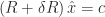
We must thus transform the perturbation in $c$ to one in $R$ . A Taylor series for the perturbation in $c$ allows us to move the perturbation from the numerator to the denominator in this way:

$\frac{1}{1+\hat{\epsilon}}=1-\epsilon+\mathcal{O\left(\epsilon^{\mathrm{2}}\right)}$

where

$\mid\hat{\epsilon}\mid\leq\epsilon_{machine}+\mathcal{O\left(\epsilon_{\mathrm{machine}}^{\mathrm{2}}\right)}$

This means that we can rewrite our equations for $\hat{x_{3}}$ as

$\hat{x_{3}}=\frac{c_{3}}{r_{3,3}\left(1+\hat{\epsilon_{3,3}}\right)}$

$\delta r_{3,3}=\hat{\epsilon_{3,3}}r_{3,3}$

Thus

$\mid\hat{\epsilon}_{3,3}\mid\leq\epsilon_{machine}+\mathcal{O\left(\epsilon_{\mathrm{machine}}^{\mathrm{2}}\right)}$

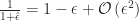
Now that we have solved for $\hat{x}_{3}$ , we can proceed up a row and solve for $\hat{x}_{2}$ . We start by solving for $\hat{x}_{2}$
as follows:

$\hat{x}_{2}=\frac{c_{2}-r_{2,3}\hat{x}_{3}}{r_{2,2}}$

Note that we have three operations in this step:

Multiplication in the numerator
Subtraction in the numerator
Division between the numerator and the denominator

This introduces three points of machine error, accounted for thus:

$\hat{x}_{2}=\frac{\left(c_{2}-r_{2,3}\hat{x}_{3}\left(1+\epsilon_{2,3}\right)\right)\left(1+\epsilon_{2,1}\right)}{r_{2,2}}\left(1+\epsilon_{2,2}\right)$

where, as always,

$\mid\epsilon_{2,1}\mid,\mid\epsilon_{2,2}\mid,\mid\epsilon_{2,3}\mid\leq\epsilon_{machine}+\mathcal{O\left(\epsilon_{\mathrm{machine}}^{\mathrm{2}}\right)}$

Using the Taylor series transformation for two out of the three error expressions,

$\hat{x}_{2}=\frac{\left(c_{2}-r_{2,3}\hat{x}_{3}\left(1+\epsilon_{2,3}\right)\right)}{r_{2,2}\left(1+\hat{\epsilon}_{2,2}\right)\left(1+\hat{\epsilon}_{2,1}\right)}$

Again,

$\mid\hat{\epsilon}_{2,1}\mid,\mid\epsilon_{2,3}\mid,\mid\hat{\epsilon}_{2,2}\mid\leq\epsilon_{machine}+\mathcal{O\left(\epsilon_{\mathrm{machine}}^{\mathrm{2}}\right)}$

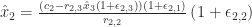
We can combine the two error expressions in the denominator by considering the fact that $\hat{\epsilon}^{2}$ is beyond our considerations, as has been consistently shown. We thus say that

$1+2\hat{\epsilon}_{2}=\left(1+\hat{\epsilon}_{2,2}\right)\left(1+\hat{\epsilon}_{2,1}\right),\mid\hat{\epsilon}_{2}\mid\leq\epsilon_{machine}+\mathcal{O\left(\epsilon_{\mathrm{machine}}^{\mathrm{2}}\right)}$

and substituting

$\hat{x}_{2}=\frac{\left(c_{2}-r_{2,3}\hat{x}_{3}\left(1+\epsilon_{2,3}\right)\right)}{r_{2,2}\left(1+2\hat{\epsilon}_{2}\right)}$

where

$\mid2\hat{\epsilon}_{2}\mid\leq2\epsilon_{machine}+\mathcal{O\left(\epsilon_{\mathrm{machine}}^{\mathrm{2}}\right)}$

Equating, as before,

$\delta r_{2,3}=\hat{\epsilon_{2,3}}r_{2,3}$

and

$\delta r_{2,2}=2\hat{\epsilon_{2}}r_{2,2}$

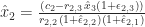
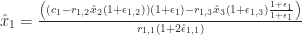
Finally we get to the top row. The value for $\hat{x}_{1}$ is given
by

$\hat{x}_{1}=\frac{\left(c_{1}-r_{1,2}\hat{x}_{2}-r_{1,3}\hat{x}_{3}\right)}{r_{1,1}}$

We have the same possibility for machine error as before, except that we have some additional calculations, each with the possibility of inducing error. Let us rewrite the above as follows:

$\hat{x}_{1}=\frac{\left(\left(c_{1}-r_{1,2}\hat{x}_{2}\right)-r_{1,3}\hat{x}_{3}\right)}{r_{1,1}}$

which more clearly shows the order of machine operations. The error points can be inserted thus:

$\hat{x}_{1}=\frac{\left(\left(c_{1}-r_{1,2}\hat{x}_{2}\left(1+\epsilon_{1,2}\right)\right)\left(1+\epsilon_{1}\right)-r_{1,3}\hat{x}_{3}\left(1+\epsilon_{1,3}\right)\right)\left(1+\epsilon_{0}\right)}{r_{1,1}}\left(1+\epsilon_{1,1}\right)$

Performing the Taylor series operation and combining $\epsilon_{0}$ and $\epsilon_{1,1}$ , we have
$\hat{x}_{1}=\frac{\left(\left(c_{1}-r_{1,2}\hat{x}_{2}\left(1+\epsilon_{1,2}\right)\right)\left(1+\epsilon_{1}\right)-r_{1,3}\hat{x}_{3}\left(1+\epsilon_{1,3}\right)\right)}{r_{1,1}\left(1+2\hat{\epsilon}_{1,1}\right)}$

Multiplying

$\hat{x}_{1}=\frac{\left(\left(c_{1}-r_{1,2}\hat{x}_{2}\left(1+\epsilon_{1,2}\right)\right)\left(1+\epsilon_{1}\right)-r_{1,3}\hat{x}_{3}\left(1+\epsilon_{1,3}\right)\frac{1+\epsilon_{1}}{1+\epsilon_{1}}\right)}{r_{1,1}\left(1+2\hat{\epsilon}_{1,1}\right)}$

Factoring out in the numerator and applying two more Taylor series transformations, we can say

$\hat{x}_{1}=\frac{\left(\left(c_{1}-r_{1,2}\hat{x}_{2}\left(1+\epsilon_{1,2}\right)\right)-r_{1,3}\hat{x}_{3}\left(1+\epsilon_{1,3}\right)\left(1+\hat{\epsilon}_{1}\right)\right)}{r_{1,1}\left(1+2\hat{\epsilon}_{1,1}\right)\left(1+\hat{\epsilon}_{1}\right)}$

Combining error terms and eliminating the squared epsilons yields

$\hat{x}_{1}=\frac{\left(\left(c_{1}-r_{1,2}\hat{x}_{2}\left(1+\epsilon_{1,2}\right)\right)-r_{1,3}\hat{x}_{3}\left(1+2\hat{\epsilon}_{1,3}\right)\right)}{r_{1,1}\left(1+3\hat{\epsilon}_{1,1}\right)}$

Noting as before that

$\delta r_{1,1}=3\hat{\epsilon_{1,1}}r_{1,1}$

$\delta r_{1,2}=\epsilon_{1,2}r_{1,2}$

$\delta r_{1,3}=\hat{2\epsilon_{1,3}}r_{1,3}$

$\mid3\hat{\epsilon}_{1,1}\mid\leq3\epsilon_{machine}+\mathcal{O\left(\epsilon_{\mathrm{machine}}^{\mathrm{2}}\right)}$

$\mid\hat{\epsilon}_{1,2}\mid\leq\epsilon_{machine}+\mathcal{O\left(\epsilon_{\mathrm{machine}}^{\mathrm{2}}\right)}$

$\mid2\hat{\epsilon}_{1,3}\mid\leq2\epsilon_{machine}+\mathcal{O\left(\epsilon_{\mathrm{machine}}^{\mathrm{2}}\right)}$

We are now able to construct the perturbation matrix thus:

$\delta R=\left[\begin{array}{ccc} 3\hat{\epsilon_{1,1}}r_{1,1} & \epsilon_{1,2}r_{1,2} & \hat{2\epsilon_{1,3}}r_{1,3}\\ 0 & 2\hat{\epsilon_{2}}r_{2,2} & \hat{\epsilon_{2,3}}r_{2,3}\\ 0 & 0 & \hat{\epsilon_{3,3}}r_{3,3} \end{array}\right]$

Now we must use this to satisfy the criterion for the backward stability of back substitution:

$\frac{\mid\delta r_{i,j}\mid}{\mid r_{i,j}\mid}\leq m\epsilon_{machine}+\mathcal{O\left(\epsilon_{\mathrm{machine}}^{\mathrm{2}}\right)}$

Let us write a matrix in accordance with this criterion and factoring
out the machine epsilon:

$\left[\begin{array}{ccc} \frac{\mid3\hat{\epsilon_{1,1}}r_{1,1}\mid}{\mid r_{1,1}\mid} & \frac{\mid\epsilon_{1,2}r_{1,2}\mid}{\mid r_{1,2}\mid} & \frac{\mid\hat{2\epsilon_{1,3}}r_{1,3}\mid}{\mid r_{1,3}\mid}\\ 0 & \frac{\mid2\hat{\epsilon_{2}}r_{2,2}\mid}{\mid r_{2,2}\mid} & \frac{\hat{\mid\epsilon_{2,3}}r_{2,3}\mid}{\mid r_{2,3}\mid}\\ 0 & 0 & \frac{\hat{\mid\epsilon_{3,3}}r_{3,3}\mid}{\mid r_{3,3}\mid} \end{array}\right]\leq\left[\begin{array}{ccc} 3 & 1 & 2\\ 0 & 2 & 1\\ 0 & 0 & 1 \end{array}\right]\epsilon_{machine}+O\left(\epsilon_{\mathrm{machine}}^{\mathrm{2}}\right)$

We can factor the machine epsilon out because we have consistently demonstrated that all of the epsilons are smaller than the machine epsilon, thus the matrix on the right hand side is greater than the one on the left. The greatest single coefficient of the machine epsilon is 3, which equals to the matrix size $m$ . So this criterion is achieved for any and all of the quotients, and thus the backward stability of back substitution is achieved.

Concerning the extension of this pattern to larger matrices, the number of errors–and thus the value of the coefficients in the normalized matrix we wrote at the end–depends upon the number of calculations and thus points of error. These can be discussed as follows:

Division: each calculation has one division. The error resulting from this division appears in the main diagonal because the denominator is always the coefficient in the diagonal, thus one error for each diagonal position is a result of the division.
Multiplication: each non-diagonal term is associated with a multiplication because we are solving for the $\hat{x}$ associated with the diagonal. So one additional error is added to each non-diagonal element in the upper portion of the matrix for multiplication.
Subtraction: there are as many subtractions as there are multiplications, but they end up in the error matrix differently. The situation with subtraction is further complicated by that fact that, in multiplying through the subtractive errors in order to get the error expressions into the denominator, the sum of the subtractive error coefficients ends up to be greater than the total number of error expressions entered into the equations. First, because of the multiplying through to get the Taylor series conversions to the denominator, the number of subtractive errors in the main diagonal (and thus associated with the denominator) is $m-i$ , where $i$ is the row number. For the rest of the matrix, the number of subtractions is $j-i-1$ , where $j$ is the column number.

The sum of any of these errors that apply to a given position in the matrix is the total number of errors in that position, and thus the value of that position in the error matrix.

The critical position is $i=j=1$ . In that position there is one error for division and $m-i$ errors for division. The sum of these is always $m$ , and thus the criterion for stability is maintained as the matrix size increased.